Parametric equations can be used to represent curves whose graphs are
not simple functions of the type y=f(x),
where y and x
are represented along the vertical and horizontal axes, respectively.
Instead, the curves in the x-y plane are defined parametrically as two
simultaneous functions of a parameter t
that ranges over some interval (minimum,
maximum). You can specify an
equation y=f(t) for the y-component
of the curve, and an equation x=g(t)
for the x-component of the curve,
for a specified range of parameter t.
Options for specifying and plotting parametric curves are available in the Custom function options pane of the 2D graph Graph Options dialog; you can also specify plots of parametric curves via the 2D Custom Function Plots options. These options are used to plot curves and functions that cannot be expressed in a simple fit of type y=f(x).
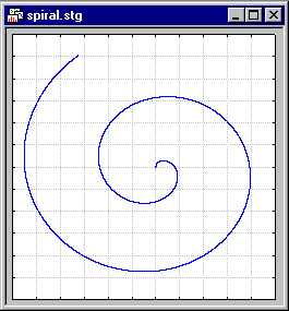
For example, to plot a spiral, you could specify:
y(t)=t*cos(t)
x(t)=t*sin(t)
For 0<=t<=12.

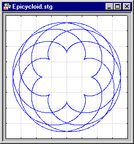
There are a wide variety of curves, from simple circles to complex shapes that can be produced via the parametric curves facilities. Here is another example:
y(t)= (a + b)*sin(t) - b*sin((a/b + 1)*t)
x(t)= (a + b)*cos(t) - b*cos((a/b + 1)* t)

In the plot shown above, a and b were set to 8 and 5, respectively, and parameter t was plotted over the range from 0 to 100. If you change a and b in the parametric equations shown above, very different shapes will emerge.