Conceptual Overviews - Quantile-Quantile Plots

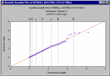
The Quantile-Quantile (or Q-Q) plot is useful for finding the best fitting distribution within a family of distributions.

The first step therefore, is to choose which of the theoretical distributions to fit to the data. After selecting the distribution from the list in the Quantile-Quantile Plots dialog, you may or may not need to specify certain parameters for that distribution.

In order to assess the fit of the theoretical distribution to the observed data, the non-missing observed values of the variable are ordered (x1 < ... < xn), and then these values (xi) are plotted against the inverse probability distribution function denoted as F-1 [specifically, F-1((i - rankadj)/(n + nadj)), where F-1 depends on the distribution, and rankadj and nadj are user-defined adjustments]. A regression line is then fit to the data in the resulting scatterplot. If the observed values fall on the regression line (fitting line), then it can be concluded that the observed values follow the specified distribution. The equation of the fitting line (Y=a + bx, given in the third title of the resulting Q-Q plot) provides parameter estimates (a and b, where a is the Threshold parameter and b is the Scale parameter) for the best fitting distribution (see the respective distribution for more information on these parameters).

For the Exponential, Extreme, Normal, and Rayleigh distributions, the standardized distribution function is used, and no additional parameters are needed.

For the Beta, Gamma, Lognormal, and Weibull distributions, the standardized distribution with specific Shape parameters is used. The Shape parameters can be specified in one of two ways:

1. The Shape parameters are user-defined (clear the Compute parameters from check box).

2. The Shape parameters are estimated (select the Compute parameters from check box) based on user-defined Threshold and Scale parameters and using either the maximum likelihood or matching moments approximation.

The Shape parameters are given in the second title of the graph.