Rod Stephens
In his April Fool’s column, Rod illustrated how to draw a “smiley face.” This month he shows you how to draw least square curves that, though less entertaining, are a bit more useful.
MANY experiments produce a set of data points. Due to the nature of the experiment, you might know (or at least suspect) that the points should lie along a straight line, even though the actual data points probably do not. In this case, you might like to find the line that best fits the data. A common way to do this is to use the method of linear least squares. [Rod’s article isn’t limited to scientific data. Consider business data that varies over time.ÑEd.]
Suppose the points (x1, y1), (x2, y2), . . ., (xN, yN) are the data points. A line that fits the data will have an equation y = m * x + b for some values of m and b.
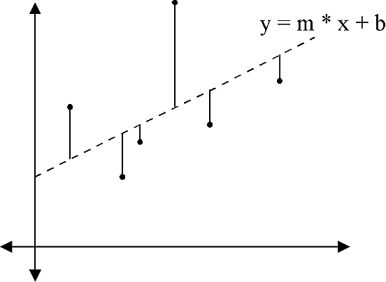
Consider one of the data points (xi, yi). The y value of the line where x = xi is given by y = m * xi + b. The vertical distance from the data point (xi, yi) to the point on the line (xi, m * xi + b) is | yi - (m * xi + b) |. If you square this number, you can drop the pesky absolute value operation because the square of a number is always positive (yi - (m * xi + b))2.
Figure 1 shows a set of data points and a line. The vertical bars show the vertical distances between the line and the points. A linear least squares fit finds the values for m and b that minimize the sum of the squares of these vertical distances for all of the data points.

Figure 1. The vertical distances between a line and data points.
Surprisingly, finding m and b isn’t too difficultÑif you remember a little calculus. Even if you don’t, you can skip the next two paragraphs and still use the equations that come later to find m and b.
Think of the sum of the squares of the distances between the points and the line as an error term E. E is a bit like an error term because it would be zero if you found a perfect fit for the data.
The equation for the error in the linear least squares method is E = S (yi - (m * xi + b))2. Here the symbol S means “the sum of.” For example, S xi means the sum of all of the xi values.
To find the minimum value of E, you take the partial derivatives of E with respect to m and b, set them equal to zero, and solve for m and b. If your calculus is a bit rusty, trust me on this step. The partial derivatives are:
¶E/¶b = S -2 * (yi - (m * xi + b))
= -2 * S (yi - m * xi - b)
= 2 * (S yi - S m * S xi - b)
¶E/¶m = S -2 * xi * (yi - (m * xi + b))
= -2 * S (xi * yi - m * xi2 - b * xi)
S1 = S 1
Sx = S xi
Sy = S yi
Sxx = S xi * xi
Sxy = S xi * yi
Then the previous equations become:
¶E/¶b = -2 * (Sy - m * Sx - b * S1)
¶E/¶m = -2 * (Sxy - m * Sxx - b * Sx)
Setting these both equal to zero and rearranging a bit you get:
Sy = m * Sx + b * S1
Sxy = m * Sxx + b * Sx
You can now solve these for m and b:
m = (S1 * Sxy - Sx * Sy) / (S1 * Sxx - Sx2)
b = (Sxx * Sy - Sx * Sxy) / ( S1 * Sxx - Sx2)
These equations look dangerous, but they’re values you can easily calculate. Remember that the (xi, yi) values are the data points that you know from the beginning. That means your program can easily calculate the sums S1, Sx, Sy, Sxx, and Sxy. Suppose the coordinates of the points are stored in the arrays PtX and PtY. Then you could use the following code to calculate the sums:
S1 = 0
Sx = 0
Sy = 0
Sxy = 0
Sxx = 0
For i = 1 To N
    S1 = S1 + 1
    Sx = Sx + PtX(i)
    Sy = Sy + PtY(i)
    Sxy = Sxy + PtX(i) * PtY(i)
    Sxx = Sxx + PtX(i) * PtX(i)
Next i
Now you can plug the sums into the equations for m and b to find the line that best fits the data points.
The file RODLEAST.ZIP, available in this month’s Subscriber Downloads at www.pinpub.com/vbd, contains the LeastSq program. LeastSq uses this technique to find a linear least squares fit to data points. Click two or more times on the picture box to select some data points and then press the Go button. The program will find and draw the line that best matches the data. Figure 2 shows the LeastSq program in action.
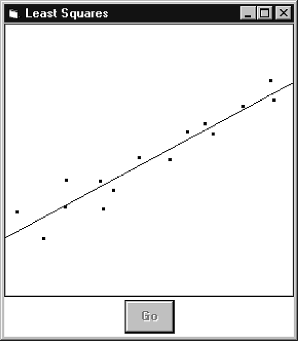
Figure 2. The LeastSq program fitting a line to some data points.
Sometimes you may know or suspect that the data points lie along a polynomial curve other than a straight line. For example, you may think the data points follow a third degree polynomial (cubic) of the form y = a * x3 + b * x2 + c * x + d. You may even suspect the points should lie along a curve of higher degree. With a little more calculus, some linear algebra, and a little patient VB coding, you can generalize the method of linear least squares for polynomials of any degree.
The general equation for a polynomial of degree D can be written like this:
y = A0 + A1 * x + A2 * x2 + ... + AD * xD
The method of polynomial least squares finds the values of the Ai that minimize the sum of the squares of the distances between the data points and this equation.
The error equation in this case is E = S (yi - (A0 + A1 * xi + A2 * xi2 + ... + AD * xiD))2. As before, you find the best values for the Ai by taking the partial derivatives of this equation with respect to each of the A’s, setting them equal to zero, and solving for the A’s. For example, here’s the partial derivative of E with respect to A1:
¶E/¶A1 = S -2 * (yi - (A0 + A1 * xi + A2 * xi2 + ... + AD * xiD)) * (xi)
= -2 * S (xi * yi - A0 * xi - A1 * xi2 - A2 * xi3 - ... - AD * xiD+1)
More generally, this is the partial derivative with respect to Aj:
¶E/¶Aj = S -2 * (yi - (A0 + A1 * xi + A2 * xi2 + ... + AD * xiD)) * (xij)
= -2 * S (xij * yi - A0 * xij - A1 * xij+1 - A2 * xij+2 - ... - AD * xij+D)
This equation seems more complicated than the previous version, but it isn’t. Remember that the values xi and yi are the constant data values that you’re trying to fit with the curve. That means terms such as xi * yi are just complicated constants that your program can calculate with a FOR loop.
If you calculate the partial derivatives with respect to each of the A’s and set them equal to zero, you’ll have D + 1 equations with D + 1 unknowns (the A’s). You can solve the equations for the A’s and get the equation for the polynomial curve.
Solving two equations with two unknowns is easy. Solving a larger system of equations isn’t too hard using Gaussian elimination (this is the linear algebra part).
First, place the equation’s coefficients in a matrix. In VB you can use a two-dimensional array. The first index in the array indicates the index of an equation. The second index is the index of a coefficient in the equation. For example, suppose you have the following K equations with K unknowns A1, A2, . . ., AK:
C00 + C01 * A1 + C02 * A2 + ... + C0K * AK = 0
C10 + C11 * A1 + C12 * A2 + ... + C1K * AK = 0
:
CK0 + CK1 * A1 + CK2 * A2 + ... + CKK * AK = 0
The array holding the coefficients would look like this:
C10 C11 C12 ... C1K
C20 C21 C22 ... C2K
: : : : :
CK0 CK1 CK2 ... CKK
The first step in Gaussian elimination is to divide each element in the first row by C11. This makes the C11 entry in the array 1. Dividing every element in the row by the same value keeps the meaning of the row unchanged. This is the same as dividing both sides of the original equation by the same value. The new and old versions are equivalent as far as determining the values of the variables is concerned.
Next, subtract a multiple of the first row from each of the others to make coefficient 1 become zero for each of the other rows. For example, coefficient 1 in the second row has value C21. If you subtract C21 times the first row from the second row, the new value for this coefficient will be C21 - C21 * 1 = 0.
Calculate the new values for the other coefficients similarly. For example, the new value for the C20 coefficient will be C20 - C21 * C10. The new value for C22 will be C22 - C21 * C12. In general, the new value for C2j will be C2j - C21 * C1j.
After you reduce every other row in this way, the first row will be the only row with a non-zero entry for coefficient 1. Now repeat the process for the other rows. Use the second row to make all of the other rows have zero for coefficient number 2. Use the third row to make all of the other rows have zero for coefficient number 3, and so forth.
One odd situation may arise during this process. You may get to a point where the coefficient that you’re trying to use to make others zero itself has the value zero. For example, suppose you’re trying to use the second row to make every other row’s coefficient number 2 have value zero, but C12 = 0. The next step at this point is to divide each element in the second row by C12. Since C12 = 0, this won’t work.
To get around this problem, swap this row with one of the later rows that has a non-zero entry in this column. This doesn’t change the meaning of the array: Each row still represents a valid equationÑthey're just stored in a different order. Eventually the array will look like this:
B00 1 0 ... 0
B10 0 1 ... 0
: : : : :
BK0 0 0 ... 1
This array corresponds to the equations:
B00 - A1 = 0
B10 - A2 = 0
:
BK0 - AK = 0
Now it’s easy to solve the equations for the unknown A’s:
A1 = -B00
A2 = -B10
:
AK = -BK0
The file ROD697.ZIP contains the Poly program. This program computes and displays polynomial least squares fits. Click several times on the picture box to select some data points. Fill in the degree the polynomial should have and press the Go button. The program will find and draw the polynomial of the given degree that best matches the data. In Figure 3 the Poly program is displaying the degree 2 (quadratic) polynomial that best fits a set of data points.
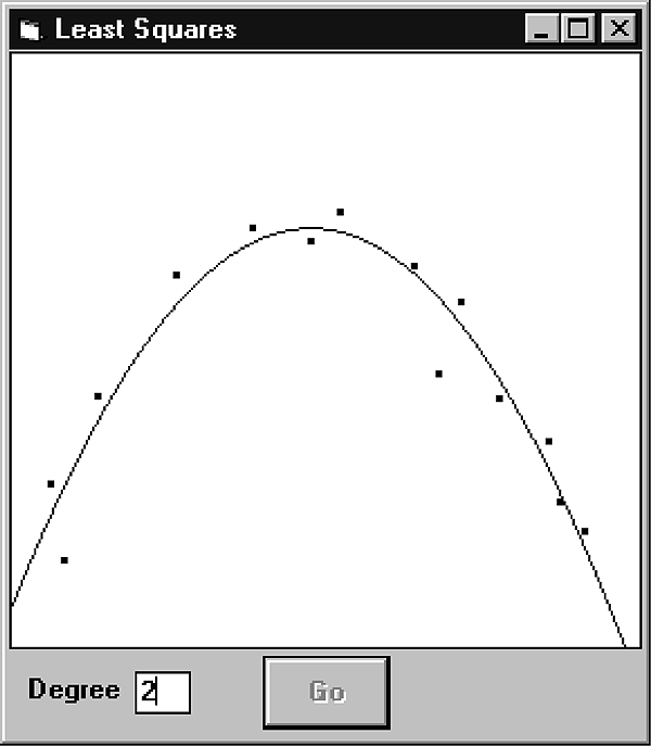
Figure 3. The Poly program that fits a quadratic curve to a set of data points.
Before you start fitting polynomials to all sorts of data values, you should be aware of a few facts.
First, a polynomial of degree D can exactly pass through D + 1 points, as long as no two points have the same X value. That means there’s no reason to use a polynomial of degree greater than D if you have only D + 1 data points. For example, a line can pass through exactly two points. If you have only two data points, there’s no reason to fit them with a degree 12 polynomial.
Second, you generally shouldn’t fit data with high-degree polynomials unless you have some reason to believe your data points were generated by a high-degree process. The higher the degree of the polynomial, the more bends the curve can make and the more closely it will fit the data. If you use a polynomial of very high degree, the curve may fit the data closely but it may hide important trends.
Figure 4 shows two curves fitting seven data points. The curve of degree six passes exactly through every point but it gives the impression that the data values wobble up and down. The degree two curve fits the points closely, though not exactly. It shows the overall structure of the data more accurately.
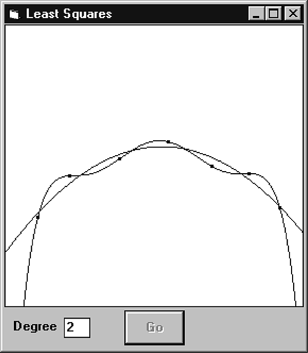
Figure 4. A high-degree curve may fit the data closely but hide more important relationships.
ROD697.ZIP at www.pinpub.com/vbd
Rod Stephens is president of Rocky Mountain Computer Consulting Inc., a custom software firm in Boulder, Colorado. His hobbies include calculus and linear algebra. He is the author of Visual Basic Algorithms and Visual Basic Graphic Programming, both from Wiley. 102124.33@compuserve.com or RodStephens@compuserve.com.
To find out more about Visual Basic Developer and Pinnacle Publishing, visit their website at: http://www.pinppub.com/vbd/
Note: This is not
a Microsoft Corporation website.
Microsoft is not responsible for its content.
This article is reproduced from the June 1997 issue of Visual Basic Developer. Copyright 1997, by Pinnacle Publishing, Inc., unless otherwise noted. All rights are reserved. Visual Basic Developer is an independently produced publication of Pinnacle Publishing, Inc. No part of this article may be used or reproduced in any fashion (except in brief quotations used in critical articles and reviews) without prior consent of Pinnacle Publishing, Inc. To contact Pinnacle Publishing, Inc., please call (800) 788-1900 or (206) 251-1900.