Plot: Fitting (3D XYZ Graphs)

These options are available in the Fitting dialog, accessible by right-clicking on a point in the graph and selecting Fitting from the shortcut menu. You can also access these options via the Graph Options dialog tree view by selecting Fitting (located under Plot).

Use these options to add a new surface to the 3D XYZ graph with the desired appearance or to modify the fitted surface by selecting the desired surface specifications. Several specifications are available to customize the axes as well as the display of the values on the modified graph.

Plot/Fit. Although all of the options are the same for each fit, you can make changes to each fit independently of the other. Use the Plot and Fit drop-down boxes to select the fit to which you want to make changes. If you have several plots in one graph, you can assign names to each plot using the Name option in the Plot: General options pane. The two fields: Plot and Fit work together. For example, to edit the third fit in plot 2, set Plot to 2 and Fit to 3. However, note that only one surface can be shown at a time (see option Display (one surface only) below).

Add new fit/Delete. Click the Add new fit button to add a new surface to your graph. When you do this, a new fit will be automatically added to the Fit box, and that new fit will be automatically selected in the Fit box. To delete a fit, select the plot that has the fit in the Plot box and the fit you want to delete in the Fit box, and click the Delete button. Note that the options here can be used for deleting fits and not plots. To delete plots, see the Plot: General options pane topic.

Display. Select the Display check box to display the surface on your graph; only the surface corresponding to the selected Plot and Fit boxes (see above) will be displayed. If you clear this check box, the surface will not be displayed at all. Note that only one surface fit can be shown per plot.

Fit type. You can fit a surface to the data in your 3D graph by selecting one of the following predefined functions from this list box:

Surface specs. Click the Surface specs button to display the Surface Specifications dialog. This dialog provides full control of the colors, shading, and other surface and contour line options that can be used to modify the appearance of your 3D graph.

Fitting data. The options under Fitting data are used to control the scale and the range of values for the axes to be used while fitting the data.

Scale. Select the scale (X, Y, or Z) from the Scale drop-down box to use in fitting the data.

Range. The Range drop-down box is used to specify the range for the selected Scale. You can choose from three ranges: Full range, Axis Range, and Custom Range. If you choose Full range, then the selected fit will be calculated using the entire range of data. If your graph has a margin around the data, the calculations for the fit will not include points that are not contained in the data. If you select Axis Range, then the fit will be calculated using the entire range of the axis, essentially using all points shown over the range of the axis. If you select Custom Range, then the fit will be calculated using the range of values specified in the Min and Max fields on this tab.

Min:, Max:. The Min and Max fields are available when you have selected Custom Range in the Range drop-down box. If this is the case, then the fit will be calculated using the range of values specified in the Min and Max fields.

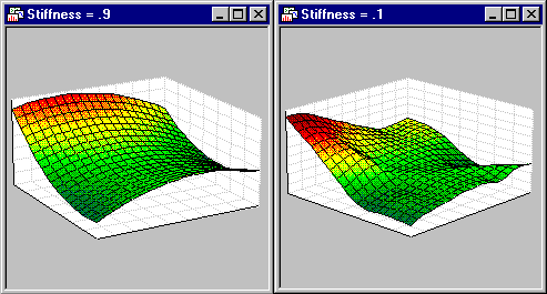
Stiffness. The weight in the Distance Weighted LS, Neg Expon Weighted LS, and Spline fits is determined by the Stiffness parameter. Specify here a value of this parameter in the range (0 < s < 1) that will determine the degree to which the fitted curve depends on the local configurations of the analyzed values.

The lower the coefficient, the more the shape of the curve is influenced by individual data points (i.e., the curve "bends" more to accommodate individual values and subsets of values). Large values of the parameter produce smoother curves that adequately represent the overall pattern in the data set at the expense of local details. The stiffness parameter is used when the Distance Weighted LS, Neg Expon Weighted LS, or Spline fit is fitted to the data (see Fit type, above). See McLain, 1974.

Value Format. Click the Value Format button to display the Value Format dialog in which you can select from a variety of value formats to use for the numeric labels. The numeric format selected here will be used, for example, in the default titles for the graph, when those titles include the fit equation for the surface shown (e.g., the equation for the Quadratic surface). For more information on these value formats see the Value Format topic.

Style. The Style drop-down box contains several predefined graphics styles from which you can choose for the selected fit. To view a menu of options related to styles (Save, Save As, Revert to unmodified, etc.), click the button next to this box.