Remember that our purpose is to measure the persons, not to optimize the items and raters. A good approach is to compute the person measures based on all the different item selections that you think are reasonable. Start with all the items, and then reduce to smaller sets of items. Cross-plot the person measures. If the person measures are collinear, use the larger set of items. If the person measures are not collinear, use the set of items which produces the more meaningful set of person measures.

 

What do Infit Mean-square, Outfit Mean-square, Infit Zstd (z-standardized), Outfit Zstd (z-standardized) mean?

 

Every observation contributes to both infit and outfit. But the weighting of the observations differs. On-target observations contribute less to outfit than to infit.

 

Outfit: outlier-sensitive fit statistic. This is based on the conventional chi-square statistic. This is more sensitive to unexpected observations by persons on items that are relatively very easy or very hard for them (and vice-versa).

 

Infit: inlier-pattern-sensitive fit statistic. This is based on the chi-square statistic with each observation weighted by its statistical information (model variance). This is more sensitive to unexpected patterns of observations by persons on items that are roughly targeted on them (and vice-versa).

 

Outfit = sum ( residual² / information ) / (count of residuals) = average ( (standardized residuals)²) = chi-square/d.f. = mean-square

 

Infit = sum ( (residual² / information) * information ) / sum(information) = average ( (standardized residuals)² * information) = information-weighted mean-square

 

Mean-square: this is the chi-square statistic divided by its degrees of freedom. Consequently its expected value is close to 1.0. Values greater than 1.0 (underfit) indicate unmodeled noise or other source of variance in the data - these degrade measurement. Values less than 1.0 (overfit) indicate that the model predicts the data too well - causing summary statistics, such as reliability statistics, to report inflated statistics. See further dichotomous and polytomous mean-square statistics.

 

Z-Standardized: these report the statistical significance (probability) of the chi-square (mean-square) statistics occurring by chance when the data fit the Rasch model. The values reported are unit-normal deviates, in which .05% 2-sided significance corresponds to 1.96. Overfit is reported with negative values. These are also called t-statistics reported with infinite degrees of freedom.

 

 

Infit was an innovation of Ben Wright's (G. Rasch, 1980, Afterword). Ben noticed that the standard statistical fit statistic (that we now call Outfit) was highly influenced by a few outliers (very unexpected observations). Ben need a fit statistic that was more sensitive to the overall pattern of responses, so he devised Infit. Infit weights the observations by their statistical information (model variance) which is higher in the center of the test and lower at the extremes. The effect is to make Infit less influenced by outliers, and more sensitive to patterns of inlying observations.

 

Ben Wright's Infit and Outfit statistics (e.g., RSA, p. 100) are initially computed as mean-square statistics (i.e., chi-square statistics divided by their degrees of freedom). Their likelihood (significance) is then computed. This could be done directly from chi-square tables, but the convention is to report them as unit normal deviates (i.e., t-statistics corrected for their degrees for freedom). I prefer to call them z-statistics, but the Rasch literature has come to call them t-statistics, so now I do to. It is confusing because they are not strictly Student t-statistics (for which one needs to know the degrees of freedom) but are random normal deviates.

 

General guidelines:

First, investigate negative point-measure or point-biserial correlations. Look at the Distractor Tables, e.g., 10.3. Remedy miskeys, data entry errors, etc.

 

Then, the general principle is:

Investigate outfit before infit,

mean-square before t standardized,

high values before low or negative values.

 

There is an asymmetry in the implications of out-of-range high and low mean-squares (or positive and negative t-statistics). High mean-squares (or positive t-statistics) are a much greater threat to validity than low mean-squares (or negative fit statistics).

 

Poor fit does not mean that the Rasch measures (parameter estimates) aren't additive. The Rasch model forces its estimates to be additive. Misfit means that the reported estimates, though effectively additive, provide a distorted picture of the data.

 

The fit analysis is a report of how well the data accord with those additive measures. So a MnSq >1.5 suggests a deviation from unidimensionality in the data, not in the measures. So the unidimensional, additive measures present a distorted picture of the data.

 

High outfit mean-squares may be the result of a few random responses by low performers. If so, drop with PDFILE= these performers when doing item analysis, or use EDFILE= to change those response to missing.

 

High infit mean-squares indicate that the items are mis-performing for the people on whom the items are targeted. This is a bigger threat to validity, but more difficult to diagnose than high outfit.

 

Mean-squares show the size of the randomness, i.e., the amount of distortion of the measurement system. 1.0 are their expected values. Values less than 1.0 indicate observations are too predictable (redundancy, model overfit). Values greater than 1.0 indicate unpredictability (unmodeled noise, model underfit). Mean-squares usually average to 1.0, so if there are high values, there must also be low ones. Examine the high ones first, and temporarily remove them from the analysis if necessary, before investigating the low ones.

 

Zstd are t-tests of the hypotheses "do the data fit the model (perfectly)?" ZSTD (standardized as a z-score) is used of a t-test result when either the t-test value has effectively infinite degrees of freedom (i.e., approximates a unit normal value) or the Student's t-statistic value has been adjusted to a unit normal value. They show the improbability (significance). 0.0 are their expected values. Less than 0.0 indicate too predictable. More than 0.0 indicates lack of predictability. If mean-squares are acceptable, then Zstd can be ignored. They are truncated towards 0, so that 1.00 to 1.99 is reported as 1. So a value of 2 means 2.00 to 2.99, i.e., at least 2. For exact values, see Output Files. If the test involves less than 30 observations, it is probably too insensitive, i.e., "everything fits". If there are more than 300 observations, it is probably too sensitive, i.e., "everything misfits".

 

 

In general, mean-squares near 1.0 indicate little distortion of the measurement system, regardless of the Zstd value.

Evaluate high mean-squares before low ones, because the average mean-square is usually forced to be near 1.0.

Mean-square fit statistics will average about 1.0, so, if you accept items (or persons) with large mean-squares (low discrimination), then you must also accept the counter-balancing items (or persons) with low mean-squares (high discrimination).

 

Outfit mean-squares:  influenced by outliers. Usually easy to diagnose and remedy. Less threat to measurement.

Infit mean-squares: influenced by response patterns. Usually hard to diagnose and remedy. Greater threat to measurement.

 

Extreme scores always fit the Rasch model exactly, so they are omitted from the computation of fit statistics. If an extreme score has an anchored measure, then that measure is included in the fit statistic computations.

 

Anchored runs: Anchor values may not exactly accord with the current data. To the extent that they don't, the fit statistics may be misleading. Anchor values that are too central for the current data tend to make the data appear to fit too well. Anchor values that are too extreme for the current data tend to make the data appear noisy.

 

Question: Are you contradicting the usual statistical advice about model-data fit?

Statisticians are usually concerned with "how likely are these data to be observed, assuming they accord with the model?" If it is too unlikely (i.e., significant misfit), then the verdict is "these data don't accord with the model." The practical concern is: "In the imperfect empirical world, data never exactly accord with the Rasch model, but do these data deviate seriously enough for the Rasch measures to be problematic?" The builder of my house followed the same approach (regarding Pythagoras theorem) when building my bathroom. It looked like the walls were square enough for his practical purposes. Some years later, I installed a full-length rectangular mirror - then I discovered that the walls were not quite square enough for my purposes (so I had to make some adjustments) - so there is always a judgment call. The table of mean-squares is my judgment call as a "builder of Rasch measures".

 

Question: Should I report Outfit or Infit?

A chi-square statistic is the sum of squares of standard normal variables. Outfit is a chi-square statistic. It is the sum of squared standardized residuals (which are modeled to be standard normal variables). So it is a conventional chi-square, familiar to most statisticians. Chi-squares (including outfit) are sensitive to outliers. For ease of interpretation, this chi-square is divided by its degrees of freedom to have a mean-square form and reported as "Outfit". Consequently I recommend that the Outfit be reported unless there is a strong reason for reporting infit.

 

In the Rasch context, outliers are often lucky guesses and careless mistakes, so these outlying characteristics of respondent behavior can make a "good" item look "bad". Consequently, Infit was devised as a statistic that downweights outliers and focuses more on the response string close to the item difficulty (or person ability). Infit is the sum of (squares of standard normal variables multiplied by their statistical information). For ease of interpretation, Infit is reported in mean-square form by dividing the weighted chi-square by the sum of the weights. This formulation is unfamiliar to most statisticians, so I recommend against reporting it unless the data are heavily contaminated with irrelevant outliers.

 

Question: Are mean-square values, >2 etc, sample-size dependent?

The mean-squares are corrected for sample size: they are the chi-squares divided by their degrees of freedom, i.e., sample size. The mean-squares answer "how big is the impact of the misfit". The t-statistics answer "how likely are data like these to be observed when the data fit the model (exactly)." In general, the bigger the sample the less likely, so that t-statistics are highly sample-size dependent. We eagerly await the theoretician who devises a statistical test for the hypothesis "the data fit the Rasch model usefully" (as opposed to the current tests for perfectly).

 

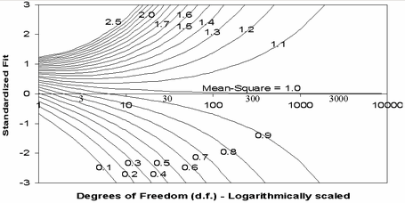
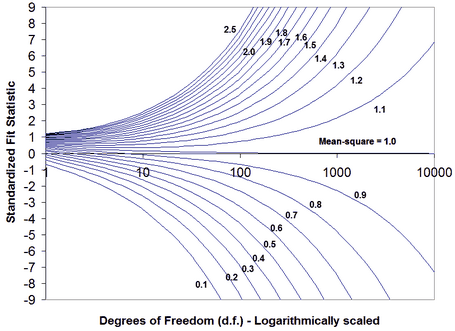
The relationship between mean-square and z-standardized t-statistics is shown in this plot. Basically, the standardized statistics are insensitive to misfit with less than 30 observations and overly sensitive to misfit when there are more than 300 observations.

 

 

Question: For my sample of 2400 people, the mean-square fit statistics are close to 1.0, but the

Z-values associated with the INFIT/OUTFIT values are huge (over 4 to 9.9). What could be causing such high values?

 

Your results make sense. Here is what has happened. You have a sample of 2,400 people. This gives huge statistically power to your test of the null hypothesis: "These data fit the Rasch model (exactly)." In the nomographs above, a sample size of 2,400 (on the right-hand-side of the plot) indicates that even a mean-square of 1.2 (and perhaps 1.1) would be reported as misfitting highly significantly. So your mean-squares tell us: "these data fit the Rasch model usefully", and the Z-values tell us: "but not exactly". This situation is often encountered in situations where we know, in advance, that the null hypothesis will be rejected. The Rasch model is a theoretical ideal. Empirical observations never fit the ideal of the Rasch model if we have enough of them. You have more than enough observations, so the null hypothesis of exact model-fit is rejected. It is the same situation with Pythagoras theorem. No empirical right-angled-triangle fits Pythagoras theorem if we measure it precisely enough. So we would reject the null hypothesis "this is a right-angled-triangle" for all triangles that have actually been drawn. But obviously billions of triangle are usefully right-angled.

 

Example of computation:

Imagine an item with categories j=0 to m. According to the Rasch model, every category has a probability of being observed, Pj.

Then the expected value of the observation is E = sum ( j * Pj )

The model variance (sum of squares) of the probable observations around the expectation is V = sum ( Pj * ( j - E ) **2 ). This is also the statistical information in the observation.

For dichotomies, these simplify to E = P1 and V = P1 * P0 = P1*(1-P1).

 

For each observation, there is an expectation and a model variance of the observation around that expectation.

residual = observation - expectation

Outfit mean-square = sum (residual**2 / model variance ) / (count of observations)

Infit mean-square = sum (residual**2) / sum (modeled variance)

 

Thus the outfit mean-square is the accumulation of squared-standardized-residuals divided by their count (their expectation). The infit mean-square is the accumulation of squared residuals divided by their expectation.

 

Outlying observations have smaller information (model variance) and so have less information than on-target observations. If all observations have the same amount of information, the information cancels out. Then Infit mean-square = Outfit mean-square.

 

For dichotomous data. Two observations: Model p=0.5, observed=1. Model p=0.25, observed =1.

Outfit mean-square = sum ( (obs-exp)**2 / model variance ) / (count of observations) = ((1-0.5)**2/(0.5*0.5)  + (1-0.25)**2/(0.25*0.75))/2 = (1 + 3)/2 = 2

Infit mean-square = sum ( (obs-exp)**2 ) / sum(model variance ) = ((1-0.5)**2 + (1-0.25)**2) /((0.5*0.5)  + (0.25*0.75)) = (0.25 + 0.56)/(0.25 +0.19) = 1.84. The off-target observation has less influence.

 

The Wilson-Hilferty cube root transformation converts the mean-square statistics to the normally-distributed z-standardized ones. For more information, please see Patel's "Handbook of the Normal Distribution" or www.rasch.org/rmt/rmt162g.htm.