(controlled by STEPT3=, STKEEP=, MRANGE=, DISCRIM=)
The average measures and category fit statistics are how the response structure worked "for this sample" (which might have high or low performers etc.). For each observation in category k, there is a person of measure Bn and an item of measure Di. Then:
average measure = sum( Bn - Di ) / count of observations in category. These are not estimates of parameters.
The probability curves are how the response structure is predicted to work for any future sample, provided it worked satisfactorily for this sample.
Our logic is that if the average measures and fit statistics don't look reasonable for this sample, why should they in any future sample? If they look OK for this sample, then the probability curves tell us about future samples. If they don't look right now, then we can anticipate problems in the future.
Persons and items with extreme scores (maximum possible and minimum possible) are omitted from Table 3.2 because they provide no information about the relative difficulty of the categories. See Table 14.3 for their details
a) For dichotomies,
SUMMARY OF CATEGORY STRUCTURE. Model="R"
FOR GROUPING "0" ACT NUMBER: 12 Go to museum
ACT DIFFICULTY MEASURE OF -1.14 ADDED TO MEASURES
-----------------------------------------------------------------------
|CATEGORY OBSERVED|OBSVD SAMPLE|INFIT OUTFIT| COHERENCE |ESTIM|
|LABEL SCORE COUNT %|AVRGE EXPECT| MNSQ MNSQ| M->C C->M RMSR |DISCR|
|-------------------+------------+------------+-----------------+-----|
| 1 1 13 17| -.45 -.06| .83 .52| 100% 23% .6686| | 1 Neutral
| 2 2 62 83| 1.06 .98| .78 .85| 86% 100% .1725| 1.23| 2 Like
-----------------------------------------------------------------------
OBSERVED AVERAGE is mean of measures in category. It is not a parameter estimate.
M->C = Does Measure imply Category?
C->M = Does Category imply Measure?
ITEM MEASURE OF -1.07 ADDED TO MEASURES
When there is only one item in a grouping (the Partial Credit model), the item measure is added to the reported measures.
CATEGORY LABEL is the number of the category in your data set after scoring/keying.
CATEGORY SCORE is the ordinal value of the category used in computing raw scores - and in Table 20.
OBSERVED COUNT and % is the count of occurrences of this category. Counts by data code are given in the distractor Tables, e.g., Table 14.3.
OBSVD AVERGE is the average of the (person measures - item difficulties) that are modeled to produce the responses observed in the category. The average measure is expected to increase with category value. Disordering is marked by "*". This is a description of the sample, not a Rasch parameter. For each observation in category k, there is a person of measure Bn and an item of measure Di. Then:
average measure = sum( Bn - Di ) / count of observations in category.
SAMPLE EXPECT is the expected value of the average measure for this sample. These values always advance with category. This is a description of the sample, not a Rasch parameter.
INFIT MNSQ is the average of the INFIT mean-squares associated with the responses in each category. The expected values for all categories are 1.0.
OUTFIT MNSQ is the average of the OUTFIT mean-squares associated with the responses in each category. The expected values for all categories are 1.0. This statistic is sensitive to grossly unexpected responses.
Note: Winsteps reports the MNSQ values in Table 3.2. An approximation to their standardized values can be obtained by using the number of observations in the category as the degrees of freedom, and then looking at the plot.
COHERENCE
M->C shows what percentage of the measures that were expected to produce observations in this category actually did. Do the measures imply the category?
Guttman's Coefficient of Reproducibility is the count-weighted average of the M->C, i.e.,
Reproducibility = sum (COUNT * M->C) / sum(COUNT * 100)
C->M shows what percentage of the observations in this category were produced by measures corresponding to the category. Does the category imply the measures?
RMSR is the root-mean-square residual, summarizing the differences between observations in this category and their expectations (excluding observations in extreme scores).
ESTIM DISCR is an estimate of the local discrimination when the model is parameterized in the form: log-odds = aj (Bn - Di - Fj)
RESIDUAL (when shown) is the residual difference between the observed and expected counts of observations in the category. Shown as % of expected, unless observed count is zero. Then residual count is shown. Only shown if residual count is >= 1.0. Indicates lack of convergence, structure anchoring, or large data set.
CATEGORY CODES and LABELS are shown to the right based on CODES=, CFILE= and CLFILE=.
Measures corresponding to the dichotomous categories are not shown, but can be computed using the Table at "What is a Logit?" and LOWADJ= and HIADJ=.
b) For rating (or partial credit) scales, the structure calibration table lists:
SUMMARY OF CATEGORY STRUCTURE. Model="R"
FOR GROUPING "0" ACT NUMBER: 1 Watch birds
ACT DIFFICULTY MEASURE OF -.89 ADDED TO MEASURES
-------------------------------------------------------------------
|CATEGORY OBSERVED|OBSVD SAMPLE|INFIT OUTFIT|| ANDRICH |CATEGORY|
|LABEL SCORE COUNT %|AVRGE EXPECT| MNSQ MNSQ||THRESHOLD| MEASURE|
|-------------------+------------+------------++---------+--------|
| 0 0 3 4| -.96 -.44| .74 .73|| NONE |( -3.66)| 0 Dislike
| 1 1 35 47| .12 .30| .70 .52|| -1.64 | -.89 | 1 Neutral
| 2 2 37 49| 1.60 1.38| .75 .77|| 1.64 |( 1.88)| 2 Like
-------------------------------------------------------------------
OBSERVED AVERAGE is mean of measures in category. It is not a parameter estimate.
ITEM MEASURE OF -.89 ADDED TO MEASURES
When there is only one item in a grouping (the Partial Credit model), the item measure is added to the reported measures.
CATEGORY LABEL, the number of the category in your data set after scoring/keying.
CATEGORY SCORE is the value of the category in computing raw scores - and in Table 20.
OBSERVED COUNT and %, the count of occurrences of this category. Counts by data code are given in the distractor Tables, e.g., Table 14.3.
OBSVD AVERGE is the average of the measures that are model led to produce the responses observed in the category. The average measure is expected to increase with category value. Disordering is marked by "*". This is a description of the sample, not the estimate of a parameter. For each observation in category k, there is a person of measure Bn and an item of measure Di. Then: average measure = sum( Bn - Di ) / count of observations in category.
SAMPLE EXPECT is the expected value of the average measure for this sample. These values always advance with category. This is a description of the sample, not a Rasch parameter.
INFIT MNSQ is the average of the INFIT mean-squares associated with the responses in each category. The expected values for all categories are 1.0. Only values greater than 1.5 are problematic.
OUTFIT MNSQ is the average of the OUTFIT mean-squares associated with the responses in each category. The expected values for all categories are 1.0. This statistic is sensitive to grossly unexpected responses. Only values greater than 1.5 are problematic.
Note: Winsteps reports the MNSQ values in Table 3.2. An approximation to their standardized values can be obtained by using the number of observations in the category as the degrees of freedom, and then looking at the plot.
ANDRICH THRESHOLD, the calibrated measure of the transition from the category below to this category. This is an estimate of the Rasch-Andrich model parameter, Fj. Use this for anchoring in Winsteps. (This corresponds to Fj in the Di+Fj parameterization of the "Rating Scale" model, and is similarly applied as the Fij of the Dij=Di+Fij of the "Partial Credit" model.) The bottom category has no prior transition, and so that the measure is shown as NONE. This parameter, sometimes called the Step Difficulty, Step Calibration, Rasch-Andrich threshold, Tau or Delta, indicates how difficult it is to observe a category, not how difficult it is to perform it. The Rasch-Andrich threshold is expected to increase with category value. Disordering of these estimates (so that they do not ascend in value up the rating scale), sometimes called "disordered deltas", indicates that the category is relatively rarely observed, i.e., occupies a narrow interval on the latent variable, and so may indicate substantive problems with the rating (or partial credit) scale category definitions. These Rasch-Andrich thresholds are relative pair-wise measures of the transitions between categories. They are the points at which adjacent category probability curves intersect. They are not the measures of the categories. See plot below.
CATEGORY MEASURE, the sample-free measure corresponding to this category. ( ) is printed where the matching calibration is infinite. The value shown corresponds to the measure .25 score points (or LOWADJ= and HIADJ=) away from the extreme. This is the best basis for the inference: "ratings averaging x imply measures of y" or "measures of y imply ratings averaging x". This is implied by the Rasch model parameters. These are plotted in Table 2.2
"Category measures" answer the question "If there were a thousand people at the same location on the latent variable and their average rating was the category value, e.g., 2.0, then where would that location be, relative to the item?" This seems to be what people mean when they say "a performance at level 2.0". It is estimated from the Rasch expectation.
We start with the Rasch model, log (Pnij / Pni(j-1) ) = Bn - Di - Fj, For known Di, Fj and trial Bn. This produces a set of {Pnij}.
Compute the expected rating score: Eni = sum (jPnij) across the categories.
Adjust Bn' = Bn + (desired category - Eni) / (large divisor), until Eni = desired category, when Bn is the desired category measure.
----------------------------------------------------------------------------------
|CATEGORY STRUCTURE | SCORE-TO-MEASURE | 50% CUM.| COHERENCE |ESTIM|
| LABEL MEASURE S.E. | AT CAT. ----ZONE----|PROBABLTY| M->C C->M RMSR |DISCR|
|------------------------+---------------------+---------+-----------------+-----|
| 0 NONE |( -3.66) -INF -2.63| | 0% 0% .9950| | 0 Dislike
| 1 -2.54 .61 | -.89 -2.63 .85| -2.57 | 69% 83% .3440| 1.11| 1 Neutral
| 2 .75 .26 |( 1.88) .85 +INF | .79 | 81% 72% .4222| 1.69| 2 Like
----------------------------------------------------------------------------------
M->C = Does Measure imply Category?
C->M = Does Category imply Measure?
CATEGORY LABEL, the number of the category in your data set after scoring/keying.
STRUCTURE MEASURE, is the Rasch-Andrich threshold, the item measure add to the calibrated measure of this transition from the category below to this category. For structures with only a single item, this is an estimate of the Rasch model parameter, Dij = Di + Fij. (This corresponds to the Dij parameterization of the "Partial Credit" model.) The bottom category has no prior transition, and so that the measure is shown as NONE. The Rasch-Andrich threshold is expected to increase with category value, but these can be disordered. "Dgi + Fgj" locations are plotted in Table 2.4, where "g" refers to the ISGROUPS= assignment. See Rating scale conceptualization.
STRUCTURE S.E. is an approximate standard error of the Rasch-Andrich threshold measure.
SCORE-TO-MEASURE
These values are plotted in Table 21, "Expected Score" ogives. They are useful for quantifying category measures. This is implied by the Rasch model parameters. See Rating scale conceptualization.
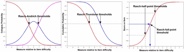
AT CAT is the Rasch-full-point-threshold, the measure (on an item of 0 logit measure) corresponding to an expected score equal to the category label, which, for the rating (or partial credit) scale model, is where this category has the highest probability. See plot below.
( ) is printed where the matching calibration is infinite. The value shown corresponds to the measure .25 score points (or LOWADJ= and HIADJ=) away from the extreme.
--ZONE-- is the Rasch-half-point threshold, the range of measures from an expected score from 1/2 score-point below to the category to 1/2 score-point above it, the Rasch-half-point thresholds. Measures in this range (on an item of 0 measure) are expected to be observed, on average, with the category value. See plot below.
50% CUMULATIVE PROBABILITY gives the location of median probabilities, i.e. these are Rasch-Thurstone thresholds, similar to those estimated in the "Graded Response" or "Proportional odds" models. At these calibrations, the probability of observing the categories below equals the probability of observing the categories equal or above. The .5 or 50% cumulative probability is the point on the variable at which the category interval begins. This is implied by the Rasch model parameters. See Rating scale conceptualization.
COHERENCE
M->C shows what percentage of the measures that were expected to produce observations in this category actually did. Do the measures imply the category?
Guttman's Coefficient of Reproducibility is the count-weighted average of the M->C, i.e., Reproducibility = sum (COUNT * M->C) / sum(COUNT * 100)
C->M shows what percentage of the observations in this category were produced by measures corresponding to the category. Does the category imply the measures?
RMSR is the root-mean-square residual, summarizing the differences between observations in this category and their expectations (excluding observations in extreme scores).
ESTIM DISCR (when DISCRIM=Y) is an estimate of the local discrimination when the model is parameterized in the form: log-odds = aj (Bn - Di - Fj)
OBSERVED - EXPECTED RESIDUAL DIFFERENCE (when shown) is the residual difference between the observed and expected counts of observations in the category. This indicates that the Rasch estimates have not converged to their maximum-likelihood values. These are shown if at least one residual percent >=1%.
residual difference % = (observed count - expected count) * 100 / (expected count)
residual difference value = observed count - expected count
1. Unanchored analyses: These numbers indicate the degree to which the reported estimates have not converged. Usually performing more estimation iterations reduces the numbers.
2. Anchored analyses: These numbers indicate the degree to which the anchor values do not match the current data.
For example,
(a) iteration was stopped early using Ctrl+F or the pull-down menu option.
(b) iteration was stopped when the maximum number of iterations was reached MJMLE=
(c) the convergence criteria LCONV= and RCONV= are not set small enough for this data set.
(d) anchor values (PAFILE=, IAFILE= and/or SAFILE=) are in force which do not allow maximum likelihood estimates to be obtained.
ITEM MEASURE ADDED TO MEASURES, is shown when the rating (or partial credit) scale applies to only one item, e.g., when ISGROUPS=0. Then all measures in these tables are adjusted by the estimated item measure.
CATEGORY PROBABILITIES: MODES - Structure measures at intersections
P ++---------+---------+---------+---------+---------+---------++
R 1.0 + +
O | |
B |00 22|
A | 0000 2222 |
B .8 + 000 222 +
I | 000 222 |
L | 00 22 |
I | 00 22 |
T .6 + 00 22 +
Y | 00 1111111 22 |
.5 + 0 1111 1111 2 +
O | 1** **1 |
F .4 + 11 00 22 11 +
| 111 00 22 111 |
R | 11 00 22 11 |
E | 111 0*2 111 |
S .2 + 111 22 00 111 +
P | 1111 222 000 1111 |
O |111 2222 0000 111|
N | 2222222 0000000 |
S .0 +22222222222222 00000000000000+
E ++---------+---------+---------+---------+---------+---------++
-3 -2 -1 0 1 2 3
PUPIL [MINUS] ACT MEASURE
Curves showing how probable is the observation of each category for measures relative to the item measure. Ordinarily, 0 logits on the plot corresponds to the item measure, and is the point at which the highest and lowest categories are equally likely to be observed. The plot should look like a range of hills. Categories which never emerge as peaks correspond to disordered Rasch-Andrich thresholds. These contradict the usual interpretation of categories as a being sequence of most likely outcomes.
Null, Zero, Unobserved Categories
STKEEP=YES and Category 2 has no observations:
+------------------------------------------------------------------
|CATEGORY OBSERVED|OBSVD SAMPLE|INFIT OUTFIT|| ANDRICH |CATEGORY|
|LABEL SCORE COUNT %|AVRGE EXPECT| MNSQ MNSQ||THRESHOLD| MEASURE|
|-------------------+------------+------------++---------+--------+
| 0 0 378 20| -.67 -.73| .96 1.16|| NONE |( -2.01)|
| 1 1 620 34| -.11 -.06| .81 .57|| -.89 | -.23 |
| 2 2 0 0| | .00 .00|| NULL | .63 |
| 3 3 852 46| 1.34 1.33| 1.00 1.64|| .89 |( 1.49)|
| 4 20 1| | || NULL | |
+------------------------------------------------------------------
Category 2 is an incidental (sampling)zero. The category is maintained in the response structure.
Category 4 has been dropped from the analysis because it is only observed in extreme scores.
STKEEP=NO and Category 2 has no observations:
+------------------------------------------------------------------
|CATEGORY OBSERVED|OBSVD SAMPLE|INFIT OUTFIT|| ANDRICH |CATEGORY|
|LABEL SCORE COUNT %|AVRGE EXPECT| MNSQ MNSQ||THRESHOLD| MEASURE|
|-------------------+------------+------------++---------+--------+
| 0 0 378 20| -.87 -1.03| 1.08 1.20|| NONE |( -2.07)|
| 1 1 620 34| .13 .33| .85 .69|| -.86 | .00 |
| 3 2 852 46| 2.24 2.16| 1.00 1.47|| .86 |( 2.07)|
+------------------------------------------------------------------
Category 2 is a structural (unobservable) zero. The category is eliminated from the response structure.
Category Misfit
Usually any MNSQ (mean-square, red box in figure) less than 2.0 is OK for practical purposes. A stricter rule would be 1.5. Overfit (values less than 1.0) are almost never a problem.
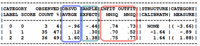
A bigger problem than category MNSQ misfit is the disordering of the "observed averages" (blue box in Figure). These contradict the Rasch axiom that "higher measure -> higher score on the rating scale".
Also large differences between the "observed average" and the "expected average" (green box in Figure). These indicate that the misfit in the category is systematic in some way.
In principle, an "expected value" is what we would see if the data fit the Rasch model. The "observed" value is what we did see. When the "observed" and "expected" are considerably misaligned, then the validity of the data (as a basis for constructing additive measures) is threatened. However, we can usually take some simple, immediate actions to remedy these defects in the data.
Usually, a 3-stage analysis suffices:
1. Analyze the data. Identify problem areas.
2. Delete problem areas from the data (PDFILE=, IDFILE=, EDFILE=, CUTLO=, etc.). Reanalyze the data. Produce item and rating-scale anchor files (IFILE=if.txt, SFILE=sf.txt) which contain the item difficulties from the good data.
3. Reanalyze all the data using the item and rating-scale anchor files (IAFILE=if.txt, SAFILE=sf.txt) to force the "good" item difficulties to dominate the problematic data when estimating the person abilities from all the data.
CategoryMnSq fit statistics
For all observations in the data:
Xni is the observed value
Eni is the expected value of Xni
Wni is the model variance of the observation around its expectation
Pnik is the probability of observing Xni=k
Category Outfit statistic for category k:
[sum ((k-Eni)²/Wni) for all Xni=k] / [sum (Pnik * (k-Eni)²/Wni) for all Xni]
Category Infit statistic for category k:
[sum ((k-Eni)²) for all Xni=k] / [sum (Pnik * (k-Eni)²) for all Xni]
Where does category 1 begin?
When describing a rating-scale to our audience, we may want to show the latent variable segmented into rating scale categories:
0-----------------01--------------------12------------------------2
There are 3 widely-used ways to do this:
1. "1" is the segment on the latent variable from where categories "0" and "1" are equally probable to where categories "1" and "2" are equally probably. These are the Rasch-Andrich thresholds (ANDRICH THRESHOLD) for categories 1 and 2.
2. "1" is the segment on the latent variable from where categories "0" and "1+2" are equally probable to where categories "0+1" and "2" are equally probably. These are the Rasch-Thurstone thresholds (50% CUM. PROBABILITY) for categories 1 and 2.
3. "1" is the segment on the latent variable from where the expected score on the item is "0.5" to where the expected score is 1.5. These are the Rasch-half-point thresholds (ZONE) for category 1.
Alternatively, we may want a point on the latent variable correspond to the category:
----------0-------------------1------------------------2-----------
4. "1" is the point on the latent variable where the expected average score is 1.0. This is the Rasch-Full-Point threshold (AT CAT.) for category 1.