Table 23.0 shows a variance decomposition of the observations for the items. This is not produced for PRCOMP=O.
Table
23.1 23.99 Tables of items with highly correlated residuals.
23.2 Plot of loadings on first contrast in residuals vs. item measures.
23.3 Items in contrast loading order.
23.4 Persons exhibiting contrast.
23.5 Items in measure order.
23.6 Items in entry order.
23.7 etc. Subsequent contrasts.
23.99 Tables of items with highly correlated residuals.
If your Table says "Total variance in observations", instead of "Total raw variance in observations", then please update to the current version of Winsteps, or produce this Table with PRCOMP=R.
Extreme items and persons (minimum possible and maximum possible raw scores) are omitted from this computation because their correlations are 0.
Simulation studies, and the empirical results of Winsteps users, indicated that the previous computation of "variance explained" was over-optimistic in explaining variance. So a more conservative algorithm was implemented. Technically, the previous computation of "variance explained" used standardized residuals (by default). These are generally considered to have better statistical properties than the raw residuals. But the raw residuals (PRCOMP=R) were found to provide more realistic explanations of variance, so the current Winsteps computation uses raw residuals for "variance explained" in the top half of the variance table.
The "Unexplained variance" is controlled by PRCOMP=, which defaults to standardized residuals (PRCOMP=S). Set PRCOMP=R to express the entire table in terms of raw residuals.
Table of STANDARDIZED RESIDUAL variance (in Eigenvalue units) |
||||
|
-- Empirical -- |
Modeled |
||
Total raw variance in observations = |
50.9 |
100.0% |
← Expected values if these data fit the Rasch model perfectly →
← If these match reasonably, then the measures explain the expected amount of variance in the data → |
100.0% |
Raw variance explained by measures = |
25.9 |
50.9% |
46.5% |
|
Raw variance explained by persons = |
10.3 |
20.2% |
18.5% |
|
Raw Variance explained by items = |
15.6 |
30.7% |
28.0% |
|
Raw unexplained variance (total) = |
25.0 = count of items (or persons) |
49.1% |
100.0% |
53.5% |
Unexplned variance in 1st contrast = |
4.6 |
9.1% |
18.5% |
← Use simulations to estimate the Rasch-model-expected values SIFILE= |
Unexplned variance in 2nd contrast = |
2.9 |
5.8% |
11.8% |
|
Unexplned variance in 3rd contrast = |
2.3 |
4.5% |
9.2% |
|
Unexplned variance in 4th contrast = |
1.7 |
3.4% |
6.9% |
|
Unexplned variance in 5th contrast = |
1.6 |
3.2% |
6.5% |
|
(More smaller contrasts) |
Eigenvalue units |
Percentage of total variance |
Percentage of unexplained variance |
|
Table of STANDARDIZED RESIDUAL variance: the standardized residuals form the basis of the "unexplained variance" computation, set by PRCOMP=
(in Eigenvalue units): variance components are rescaled so that the total unexplained variance has its expected summed eigenvalue.
Empirical: variance components for the observed data
Model: variance components expected for these data if they exactly fit the Rasch model, i.e., the variance that would be explained if the data accorded with the Rasch definition of unidimensionality.
Total raw variance in observations: total raw-score variance in the observations
Raw variance explained by measures: raw-score variance in the observations explained by the Rasch item difficulties, person abilities and rating scale structures
Raw variance explained by persons: raw-score variance in the observations explained by the Rasch person abilities (and apportioned rating scale structures)
Raw variance explained by items: raw-score variance in the observations explained by the Rasch item difficulties (and apportioned rating scale structures)
Raw unexplained variance (total): raw-score variance in the observations not explained by the Rasch measures
Unexplned variance in 1st, 2nd, ... contrast: size of the first, second, ... contrast (component) in the principal component decomposition of standardized residuals (or as set by PRCOMP=), i.e., variance that is not explained by the Rasch measures, but that is explained by the contrast.
The important lines in this Table are "contrasts". If the first contrast is much larger than the size of an Eigenvalue expected by chance, usually less than 2 - www.rasch.org/rmt/rmt191h.htm - please inspect your Table 23.3 to see the contrasting content of the items which is producing this large off-dimensional component in your data, or Table 24.3 to see the contrasting persons. The threat to Rasch measurement is not the ratio of unexplained (by the model) to explained (by the model), or the amount of explained or unexplained. The threat is that there is another non-Rasch explanation for the "unexplained". This is what the "contrasts" are reporting.
How Variance Decomposition is done ...
| 1. | A central person ability and a central item difficulty are estimated. When the central ability is substituted for the estimated person abilities for each observation, the expected total score on the instrument across all persons equals the observed total score. Similarly, when the central ability is substitute for the estimated item difficulties for each observation, the expected total score on the instrument across all items equals the observed total score. |
| 2. | For each observation, a central value is predicted from the central person ability and the central item difficulty and the estimated rating scale (if any). In the "Empirical" columns: |
| 3. | "Total raw variance in observations =" the sum-of-squares of the observations around their central values. |
| 4. | "Raw unexplained variance (total)=" is the sum-of-squares of the difference between the observations and their Rasch predictions, the raw residuals. |
| 5. | "Raw variance explained by measures=" is the difference between the "Total raw variance" and the "Raw unexpained variance". |
| 6. | "Raw variance explained by persons=" is the fraction of the "Raw variance explained by measures=" attributable to the person measure variance (and apportioned rating scale structures). |
| 7. | "Raw variance explained by items=" is the fraction of the "Raw variance explained by measures=" attributable to the item measure variance (and apportioned rating scale structures). |
| 8. | The reported variance explained by the items and the persons is normalized to equal the variance explained by all the measures. This apportions the variance explained by the rating scale structures. |
| 9. | The observation residuals, as transformed by PRCOMP=, are summarized as an inter-person correlation matrix, with as many columns as there are non-extreme persons. This correlation matrix is subjected to Principle Components Analysis, PCA. |
| 10. | In PCA, each diagonal element (correlation of the person with itself) is set at 1.0. Thus the eigenvalue of each person is 1.0, and the total of the eigenvalues of the matrix is the number of persons. This is the sum of the variance modeled to exist in the correlation matrix, i.e., the total of the unexplained variance in the observations. |
| 11. | For convenience the size of the "Raw unexplained variance (total)" is rescaled to equal the total of the eigenvalues. This permits direct comparison of all the variance terms. |
| 12. | The correlation matrix reflects the Rasch-predicted randomness in the data and also any departures in the data from Rasch criteria, such as those due to multidimensionality in the persons. |
| 13. | PCA reports components. If the data accord with the Rasch model, then each person is locally independent and the inter-person correlations are statistically zero. The PCA analysis would report each person as its own component. Simulation studies indicate that even Rasch-conforming data produce eigenvalues with values up to 2.0, i.e., with the strength of two persons. |
| 14. | Multidimensionality affects the pattern of the residuals. The residual pattern should be random, so the "contrast" eigenvalue pattern should approximately match the eigenvalue pattern from simulated data. When there is multidimensionality the residuals align along the dimensions, causing the early contrast eigenvalues to be higher than those from random (simulated) data. So multidimensionality inflates the early PCA contrasts above the values expected from random data, and correspondingly must lower the later ones, because the eigenvalue total is fixed. |
| 15. | "Unexplned variance in 1st contrast =" reports the size of the first PCA component. This is termed a "contrast" because the substantive differences between persons that load positively and negatively on the first component are crucial. It may reflect a systematic second dimension in the persons. |
| 16. | "Unexplned variance in 2nd contrast =". Consecutively smaller contrasts are reported (up to 5 contrasts). These may also contain systematic multi-dimensionality in the persons. In the "Model" columns: |
| 17. | "Raw variance explained by measures=" is the sum-of-squares of the Rasch-predicted observations (based on the item difficulties, person abilities, and rating scale structures) around their central values. |
| 18. | "Raw variance explained by persons=" is the fraction of the "Raw variance explained by measures=" attributable to the person measure variance (and apportioned rating scale structures). |
| 19. | "Raw variance explained by items=" is the fraction of the "Raw variance explained by measures=" attributable to the item measure variance (and apportioned rating scale structures). |
| 20. | The reported variance explained by the items and the persons is normalized to equal the variance explained by all the measures. This apportions the variance explained by the rating scale structures. |
| 21. | "Raw unexplained variance (total)=" is the summed Rasch-model variances of the observations around their expectations, the unexplained residual variance predicted by the Rasch model. |
| 22. | "Total raw variance in observations =" is the sum of the Rasch-model "Raw variance explained by measures=" and the "Raw unexplained variance (total)=" |
| 23. | The "Model" and the "Empirical" values for the "Total raw variance in observations =" are both rescaled to be 100%. |
| 24. | Use the SIFILE= option in order to simulate data. From these data predicted model values for the contrast sizes can be obtained. |
STANDARDIZED RESIDUAL VARIANCE SCREE PLOT
VARIANCE COMPONENT SCREE PLOT +--+--+--+--+--+--+--+--+--+--+--+ 100%+ T + | | V 63%+ + A | M | R 40%+ U + I | | A 25%+ I + N | P | C 16%+ + E | | 10%+ + L | 1 | O 6%+ + G | 2 | | 4%+ 3 + S | 4 5 | C 3%+ + A | | L 2%+ + E | | D 1%+ + | | 0.5%+ + +--+--+--+--+--+--+--+--+--+--+--+ TV MV PV IV UV U1 U2 U3 U4 U5 VARIANCE COMPONENTS |
Scree plot of the variance component percentage sizes, logarithmically scaled:
On plot |
On x-axis |
Meaning |
T |
TV |
total variance in the observations, always 100% |
M |
MV |
variance explained by the Rasch measures |
P |
PV |
variance explained by the person abilities |
I |
IV |
variance explained by the item difficulties |
U |
UV |
unexplained variance |
1 |
U1 |
first contrast (component) in the residuals |
2 |
U2 |
second contrast (component) in the residuals, etc. |
For the observations (PRCOMP=Obs), a standard Principal Components Analysis (without rotation, and with orthogonal axes) is performed based on the scored observations.
Table of OBSERVATION variance (in Eigenvalue units)
-- Empirical --
Raw unexplained variance (total) = 13.0 100.0%
Unexplned variance in 1st contrast = 9.9 76.1%
Unexplned variance in 2nd contrast = .9 7.2%
Unexplned variance in 3rd contrast = .6 4.3%
Unexplned variance in 4th contrast = .3 2.6%
Unexplned variance in 5th contrast = .3 2.0%
Here "contrast" means "component" or "factor".
Example 1:
We are trying to explain the data by the estimated Rasch measures: the person abilities and the item difficulties. The Rasch model also predicts random statistically-unexplained variance in the data. This unexplained variance should not be explained by any systematic effects.
Table of RAW RESIDUAL variance (in Eigenvalue units)
Empirical Modeled
Total raw variance in observations = 19.8 100.0% 100.0%
is composed of
Raw variance explained by measures = 7.8 39.3% 39.1%
Raw unexplained variance (total) = 12.0 60.7% 100.0% 60.9%
Nothing is wrong so far. The measures are central, so that most of the variance in the data is unexplained. The Rasch model predicts this unexplained variance will be random.
Raw variance explained by measures = 7.8 39.3% 39.1%
is composed of
Raw variance explained by persons = 5.7 28.9% 28.8%
Raw Variance explained by items = 2.1 10.4% 10.3%
Nothing is wrong so far. The person measures explain much more variance in the data than the item difficulties. This is probably because the person measure S.D. is bigger than the item difficulty S.D. in Table 3.1.
Raw unexplained variance (total) = 12.0 60.7% 100.0% 60.9%
is composed of
Unexplned variance in 1st contrast = 2.6 13.1% 21.5%
Unexplned variance in 2nd contrast = 1.4 6.9% 11.4%
Unexplned variance in 3rd contrast = 1.3 6.4% 10.6%
Unexplned variance in 4th contrast = 1.1 5.6% 9.3%
Unexplned variance in 5th contrast = 1.1 5.4% 8.9%
(and about 7 more)
Now we have multidimensionality problems. According to Rasch model simulations, it is unlikely that the 1st contrast in the "unexplained variance" (residual variance) will have a size larger than 2.0. Here it is 2.6. Also the variance explained by the 1st contrast is 13.1%. this is larger than the variance explained by the item difficulties 10.4%. A secondary dimension in the data appears to explain more variance than is explained by the Rasch item difficulties. Below is the scree plot showing the relative sizes of the variance components (logarithmically scaled).
VARIANCE COMPONENT SCREE PLOT
+--+--+--+--+--+--+--+--+--+--+--+
100%+ T +
| |
V 63%+ +
A | U |
R 40%+ +
I | M |
A 25%+ P +
N | |
C 16%+ +
E | 1 |
10%+ I +
L | |
O 6%+ 2 3 +
G | 4 5 |
| 4%+ +
S | |
C 3%+ +
A | |
L 2%+ +
E | |
D 1%+ +
| |
0.5%+ +
+--+--+--+--+--+--+--+--+--+--+--+
TV MV PV IV UV U1 U2 U3 U4 U5
VARIANCE COMPONENTS
Example 2:
Question: My Rasch dimension only explains 45.5% of the variance in the data and there is no clear secondary dimension. How can I increase the "variance explained"?
Reply: If there is "no clear secondary dimension" and no excessive amount of misfitting items or persons, then your data are under statistical control and your "variance explained" is as good as you can get without changing the sample or the instrument.
Predicted Explained-Variance
A Rasch model predicts that there will be a random aspect to the data. This is well understood. But what does sometimes surprise us is how large the random fraction is. The Figure shows the proportion of "variance explained" predicted to exist in dichotomous data under various conditions.
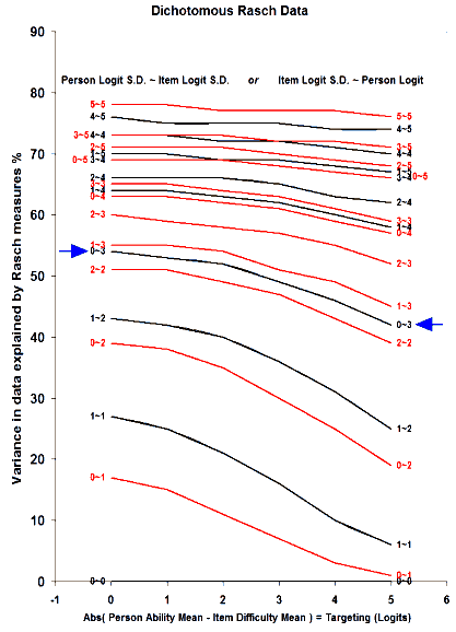
The x-axis is the absolute difference between the mean of the person and item distributions, from 0 logits to 5 logits. The y-axis is the percent of variance in the data explained by the Rasch measures. Each plotted line corresponds to one combination of standard deviations. The lesser of the person S.D. and the item S.D. is first, 0 to 5 logits, followed by "~". Then the greater of the person S.D. and the item S.D. Thus, the arrows indicate the line labeled "0-3". This corresponds to a person S.D. of 0 logits and an item S.D. of 3 logits, or a person S.D. of 0 logits and an item S.D. of 3 logits. The Figure indicates that, with these measure distributions about 50% of the variance in the data is explained by the Rasch measures. When the person and item S.D.s, are around 1 logit, then only 25% of the variance in the data is explained by the Rasch measures, but when the S.D.s are around 4 logits, then 75% of the variance is explained. Even with very wide person and item distributions with S.D.s of 5 logits only 80% of the variance in the data is explained.
In general, to increase the variance explained, there must be a wide range of person measures and/or of item difficulties. We can obtain this in three ways:
1. Increase the person S.D.: Include in the sample more persons with measures less central than those we currently have (or omit from the sample persons with measures in the center of the person distribution)
2. Increase the item S.D.: Include in the test more items with measures less central than those we currently have (or omit from the test items with measures in the center of the item distribution)
3. Make the data more deterministic (Guttman-like) so that the estimated Rasch measures have a wider logit range:
a.) Remove "special causes" (to use quality-control terminology) by trimming observations with extreme standardized residuals.
b.) Reduce "common causes" by making the items more discriminating, e.g., by giving more precise definitions to rating scale categories, increasing the number of well-defined categories, making the items more similar, etc.
However, for a well-constructed instrument administered in a careful way to an appropriate sample, you may already be doing as well as is practical.
For comparison, here are some percents for other instruments: |
||
exam12.txt |
78.7% |
(FIM sample chosen to exhibit a wide range of measures) |
exam1.txt |
71.1% |
(Knox Cube Test) |
example0.txt |
50.8% |
(Liking for Science) |
interest.txt |
37.5% |
(NSF survey data - 3 category rating scale) |
agree.txt |
30.0% |
(NSF survey data - 4 category rating scale) |
exam5.txt |
29.5% |
(CAT test) - as CAT tests improve, this % will decrease! |
coin-toss |
0.0% |
|
In Winsteps Table 23.0, the "Model" column gives the "Variance Explained" value that you could expect to see if your data had perfect fit to the Rasch model with the current degree of randomness. The "Model" value is usually very close to the empirical value. This is because some parts of your data underfit the model (too little variance explained) and some parts overfit (too much variance explained).
Relationship to Bigsteps and earlier versions of Winsteps:
My apologies for the difficulties caused by the change in computation to "Variance Explained".
The earlier computation was based on the best statistical theory available to us at the time. Further developments in statistical theory, combined with practical experience, indicated that the previous computation was too generous in assigning "variance explained" to the Rasch measures. The current computation is more accurate.
Set PRCOMP=R (raw residuals) in Bigsteps and earlier versions of Winsteps, and you will obtain approximately the same explained/unexplained variance proportions as the current version of Winsteps.
Research in the last couple of years has demonstrated that PRCOMP=R gives a more realistic estimate of the variance explained than PRCOMP=S (standardized residuals). PRCOMP=S overestimates the explained variance as a proportion of the total variance.
But for decomposing the unexplained variance into "contrasts", PRCOMP=S is better. So this mixed setting is now the default for Winsteps.
The Eigenvalue reported for the 1st contrast has not changed. If this is much larger than the size of an Eigenvalue expected by chance, usually less than 2 - www.rasch.org/rmt/rmt191h.htm - Please inspect your Table 23.3 to see the contrasting content of the items which is producing this large off-dimensional component in your data.