In Rasch analysis, we use item correlations as an immediate check that the response-level scoring makes sense. If the observed correlation is negative, something may have gone wrong (MCQ miskey, reversed survey item, etc.)
In general, correlations are much too difficult to interpret, so we switch over to using mean-squares. The "expected correlation" indicates when conventional rules such as eliminate items with point-biserials less than 0.2 are misleading.
Item correlations are difficult to interpret because they are influenced by:
1. predictability of the data
2. targeting of the item on the person sample
3. distribution of the person sample
In Rasch analysis, we are chiefly concerned about the predictability of the data when assessing item quality, so we examine the predictability directly using the mean-square statistics, rather than indirectly through the correlations.
All correlations are computed as Pearson product-moment correlation coefficients. If you wish to compute other correlations, the required data are in XFILE= IPMATRIX=, IFILE= or PFILE=. The Biserial correlation can be computed from the point-biserial.
In Table 14.1 and other measure Tables:
Point-Biserial Correlations (for dichtomies, and Point-Polyserial for polytomies)
when PTBISERIAL=Yes
PTBSE is the point-biserial correlation between the responses to this item by each person and the total marginal score by each person (omitting the response to this item). This is the "point-biserial corrected for spuriousness". Henrysson, S. (1963). Correction for item-total correlations in item analysis. Psychometrika, 28, 211-218.
when PTBISERIAL=All
PTBSA is the point-biserial correlation between the responses to this item by each person and the total marginal score by each person (including the response to this item). This is the conventional point-biserial.
In Table 14.3 and other or distractor Tables:
when PTBISERIAL=Yes or PTBISERIAL=All
PTBSD is the distractor point-biserial correlation between the indicated response to this item (scored 1 and other responses scored 0) by each person and the total marginal score by each person.
There is a closer match between Table 14.1 and Table 14.3 when PTBISERIAL=All
PTBIS=Y or E (indicated by PTBSE): The point-biserial correlation rpbis for item i (when i=1,L for persons n=1,N) is the correlation between the observation for each person on item i and the total score for each person on all the items excluding item i (and similarly for the point-biserial for each person):

PTBIS=All (indicated by PTBSA): All the observations are included in the total score:
where X1,..,XN are the responses, and Y1,..,YN are the total scores. The range of the correlation is -1 to +1.
Under classical (raw-score) test theory conventions, point-biserial correlations should be 0.3, 0.4 or better. Under Rasch conditions, point-biserial (or point-measure) correlations should be positive, so that the item-level scoring accords with the latent variable, but the size of a positive correlation is of less importance than the fit of the responses to the Rasch model, indicated by the mean-square fit statistics.
Point-Measure Correlations
PTBIS=No (indicated by PTMEA): The correlation between the observations and the Rasch measures:
where X1,..,XN are the responses by the persons (or on the items), and Y1,..,YN are the person measures (or the item easinesses = - item difficulties). The range of the correlation is -1 to +1.
Jaspen, N. (1946) "Serial Correlation", Psychometrika, 11, 23-30.
Olsson, U., Drasgow, F. and Dorans, N.J. (1982) "The Polyserial Correlation Coefficient", Psychometrika, 47, 337-347.
The Expected Value of a Correlation
Interpreting an observed value is made easier if we can compare it with its expected value. Is is much higher than expected or much lower than expected?
The general formula for a Pearson correlation coefficient is shown above. Suppose that Xn is Xni the observation of person n on item i. Yn is Bn the ability of person n, then the point-measure correlation is:
According to the Rasch model, the expected value of Xni is Eni and its model variance around the expectation is Wni where Sum(Eni) = Sum(Xni) for n=1,N. Thus an estimate of the expected value of the point-measure correlation is given by the Rasch model proposition that: Xni = Eni ±√Wni. Other variance terms are much smaller.
±√Wni is a random residual with mean 0 and variance Wni. Its value for any observation is known: Wni = Eni(1-Eni) for dichotomies. Its cross-product with any other variable is modeled to be zero. Thus, simplifying,
and similarly for the point-biserial correlations. Here is an example with an Excel spreadsheet:
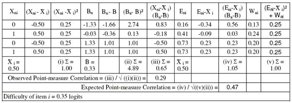
Figure courtesy of Peter Karaffa
Disattenuated correlation coefficients
"Attenuated" means "reduced". "Disattenuation" means "remove the attenuation".
The observed correlation between two variables is attenuated (reduced toward zero) because the variables are measured with error. So, when we remove the measurement error (by a statistical operation), the resulting correlation is disattenuated. Disattenuated correlations are always further from zero.
Algebraically:
{A} and {B} are the "true" values of two variables. Their true (disattenuated) correlation is
Disattenuated ("true") correlation = r(A,B)
But the observed values of the variables are measured with error {A±a}, {B±b}, so the observed correlation is
observed correlation = r(A,B) * √(var(A)*var(B))/√((var(A)+a²)*(var(B)+b²)).
"Disattenuation" reverses this process.
If the reliability of {A} is RA, and the reliability of {B} is RB, then the disattenuated correlation between {A} and {B} is:
disattenuated r(A,B) = r(A,B) / √(RA*RB).