From the Plots menu, this enables the simple graphical or tabular comparison of equivalent statistics from two runs using a scatterplot (xyplot).
To automatically produce this Excel scatterplot of two sets of measures or fits statistics:
Select Compare Statistics on the Plots pull-down menu. If this dialog box is too big for your screen see Display too big.
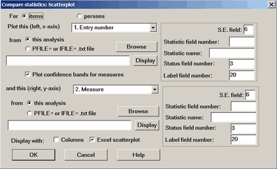
Measures, standard errors, fit statistics indicate which statistics are to be compared.
Display with columns generates a line-printer graphical-columns plot. It is displayed as Table 34.
The first column is the Outfit Mean-Square of this analysis.
The third column is the Outfit Mean-Square of the Right File (exam12lopf.txt in this case)
The second column is the difference.
The fourth column is the identification, according to the current analysis.
Persons or items are matched and listed by Entry number.
Table 34.1
+-----------------------------------------------------------------------------+
| PERSON | Outfit MnSq Difference | exam12lopf.txt | File Compa|
|0 1 3|-2 0 2|0 1 3| NUM LABEL|
|-------------------+-------------------------+-------------------+-----------|
| . * | * . | * . | 1 21101 |
| . * | * . | . * | 2 21170 |
| * . | .* | * . | 3 21174 |
....
| *. | * | *. | 35 22693 |
+-----------------------------------------------------------------------------+
Display with Excel scatterplot initiates a graphical scatterplot plot. If the statistics being compared are both measures, then a 95% confidence interval is shown. This plot can be edited with all Excel tools.
Comparing with files
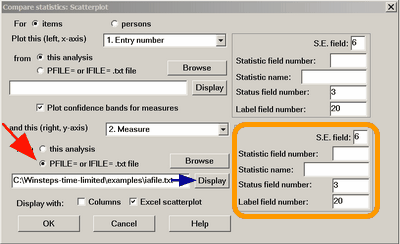
One or both sets of statistics can be in a IFILE= or PFILE= file (red arrow). Since these files can have different formats, please check that the selected field number matches the correct field in your file by clicking on the Display button (blue arrow). This displays the file. Count across the numerical fields to your selected statistic. If your field number differs from the standard field number, please provide the correct details for your field in the selection box (orange box).
There are several decisions to make:
1. Do you want to plot person (row) or item (column) statistics?
2. Which statistic for the x-axis?
3. Which statistic for the y-axis?
4. Do you want to use the statistic from this analysis or from the PFILE= or IFILE= of another analysis?
5. Do you want to display in the statistics as Columns in a Table or as an Excel scatterplot or both?
If you are using the statistic from a PFILE= or IFILE= and Winsteps selects the wrong column, then identify the correct column using the "Statistic field number" area.
When two measures are compared, then their standard errors are used to construct confidence bands when "Plot confidence bands" is checked:
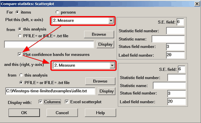
Here the item calibrations in the current analysis are being compared with the item calibrations in file IFILE=SFIF.txt from another analysis. This is the columnar output:
TABLE 34.1 An MCQ Test: administration was Comput ZOU630WS.TXT Apr 21 2:21 2006
INPUT: 30 STUDENTS 69 TOPICS REPORTED: 30 STUDENTS 69 TOPICS 2 CATS 3.60.2
--------------------------------------------------------------------------------
+----------------------------------------------------------------------------------------------------+
| Measures | Differences | Measures | Comparison |
| | | SFIF.txt | |
|-4 1|-2 5|-3 2| NUM TOPIC |
|-------------------+--------------------------+-------------------+---------------------------------|
| * . | . * | *. | 1 nl01 Month |
| . * | * . | * . | 2 nl02 Sign |
| * . | . * | .* | 3 nl03 Phone number |
| * . | . * | . * | 4 nl04 Ticket |
| * . | . *| . *| 5 nl05 building |
|* . | . * | .* | 6 nm01 student ticket |
| * . | . * | . * | 7 nm02 menu |
| * . | . * | . * | 8 nm03 sweater |
| * . | . * | . * | 9 nm04 Forbidden City |
| * . | . * | * . | 10 nm05 public place |
| * . | . * | * . | 11 nm06 post office |
| * . | . * | * . | 12 nm07 sign on wall |
| * . | * | * . | 13 nh01 supermarket |
| * . | . * | .* | 14 nh02 advertisement |
| .* | * . | * . | 15 nh03 vending machine |
| * . | . * | .* | 16 nh04 outside store |
| * | * | * | 17 nh05 stairway |
| * . | * . | * . | 18 nh06 gas station |
| * . | * . | * . | 19 nh07 Taipei |
| * . | . * | . * | 20 nh08 window at post office |
| * | * . | * . | 21 nh09 weather forecast |
| * . | . * | * | 22 nh10 section of newspaper |
| * . | . * | . * | 23 nh11 exchange rate |
| *. | * | *. | 24 il01 open |
| * . | . * | .* | 25 il02 vending machine |
+----------------------------------------------------------------------------------------------------+
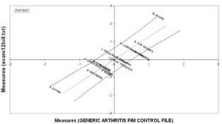
and the plotted output:
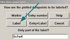
We are selecting only the first 4 characters of the item label, e.g., "nl01" and plotting only the Label:
1. Plots with confidence bands:
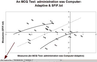
The points are plotted by their labels. The curved lines are the approximate 95% two-sided confidence bands (smoothed across all the points). They are not straight because the standard errors of the points differ. In this plot called "Plot-Empirical line" (red arrow), the dotted line is the empirical equivalence (best-fit) line. Right-click on a line to reformat or remove it.
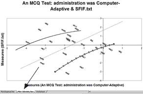
A line parallel to the identity line is shown on the "Plot-Identity line" (blue arrow) by selecting the tab on the bottom of the Excel screen. This line is parallel to the standard identity line (of slope 1), but goes through the origin of the two axes. This parallel-identity line goes through the mean of the two sets of measures (vertical and horizontal).
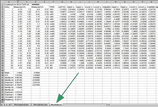
The plotted points are in the Excel Worksheet (green arrow). You can edit the data points and make any other changes you want to the plots.
The relationship between the variables is summarized in the lower cells.
Empirical slope = S.D.(y-values) / S.D.(x-values)
Intercept = intersection of the line with empirical slope through the point: mean(x-values), mean(y-values)
Predicted y-value = intercept with y-axis + x-value * empirical slope
Predicted x-value = intercept with x-axis + y-value / empirical slope
Disattenuated correlation approximates the "true" correlation without measurement error.
Disattenuated correlation = Correlation / sqrt (Reliability(x-values) * Reliability(y-values))
In Row 1, the worksheet allows for user-adjustable confidence bands.
2. Plots without confidence bands
The plot can be edited with the full functionality of Excel.
The Worksheet shows the correlation of the points on the two axes.
![]()